
The AI doesn't just fit the data — it discovers the equation.
Real models are partly known: you have the physics for most of a system and a gap where the physics is wrong or missing. A black-box neural network fits the training window, extrapolates badly, and tells you nothing. A Universal Differential Equation keeps every term you know, drops a neural network into only the unknown channel, trains the hybrid model through the ODE solver, and then reads the learned gap back as a symbolic equation by sparse regression. This program runs that loop end to end on the Julia SciML stack — and signs it off.
You rarely know all the physics — and rarely none.
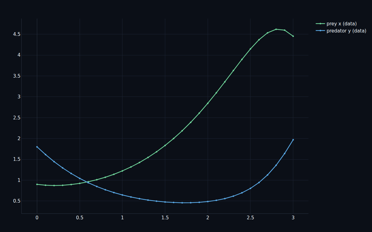
The hero system is Lotka-Volterra predator-prey, with the bilinear interaction term treated as the unknown physics: the linear birth and death rates are known, the coupling that makes the populations oscillate is not. That's the realistic case — a mechanistic skeleton with a hole in it. Drop the interaction and the model collapses (prey explode, predators die out); the closed-orbit data is what a learner has to reconstruct the missing closure from.
A black box fits the window and fails the moment it leaves it.
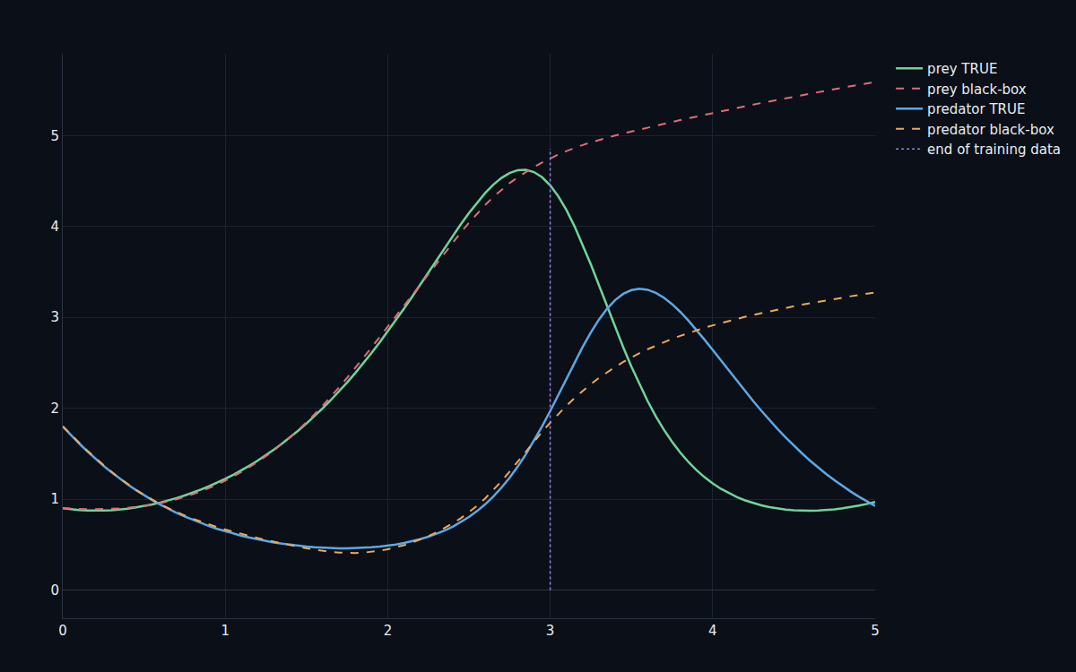
The obvious move is to learn the whole right-hand side with a neural network — a neural ODE. It works inside the training window (fit RMSE 0.053) and is completely useless outside it: extrapolation error jumps 52× and the trajectory drifts off the data manifold entirely. It also can't tell you anything — there's no equation to read, no physics to check. That failure is the whole reason to keep the physics you already have.
Keep the physics, learn only the gap — through the solver.
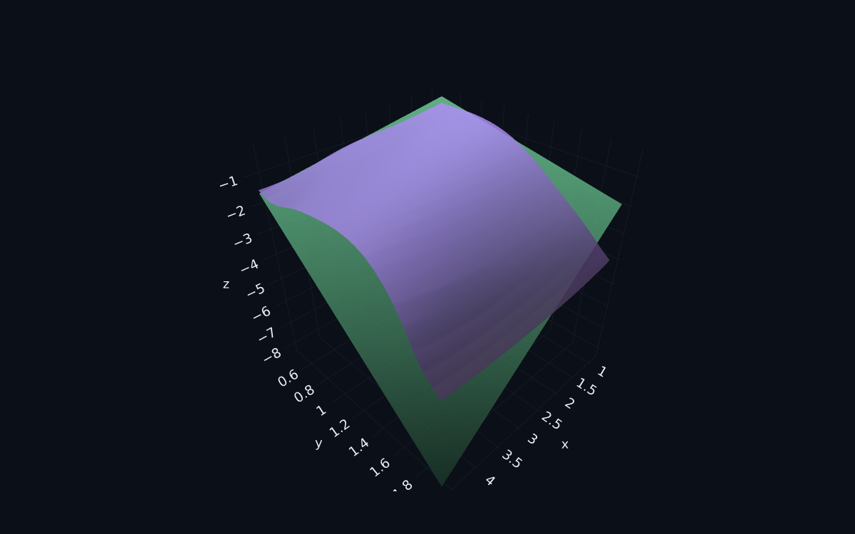
The Universal Differential Equation writes the right-hand side as the known linear terms plus a neural network in only the unknown interaction channel, and trains it through the ODE solver itself — continuous adjoint sensitivities (InterpolatingAdjoint + a Zygote vector-Jacobian product), the Lux parameters flattened to a plain vector so the adjoint sees them. The trajectory loss falls from 2.4 to 0.0085 over 1500 steps; the hybrid model fits to RMSE 0.065. And because the network sits in a known place, you can look at what it learned: the learned interaction surface matches the true −b·xy term with correlation 0.926 / 0.958.
Read the learned term back as an equation.
The learned term is a smooth function in a known channel — so it can be turned back into symbols. Sampling the dynamic residual (measured derivative minus the known part) across a small ensemble of orbits and sparse-regressing it onto a polynomial library with sequential thresholded least-squares recovers exactly the terms that belong: −0.9·xy for the prey, +0.8·xy for the predator, every other candidate driven to zero — 0.0% coefficient error. That's not a fit; it's the governing equation, discovered from data.
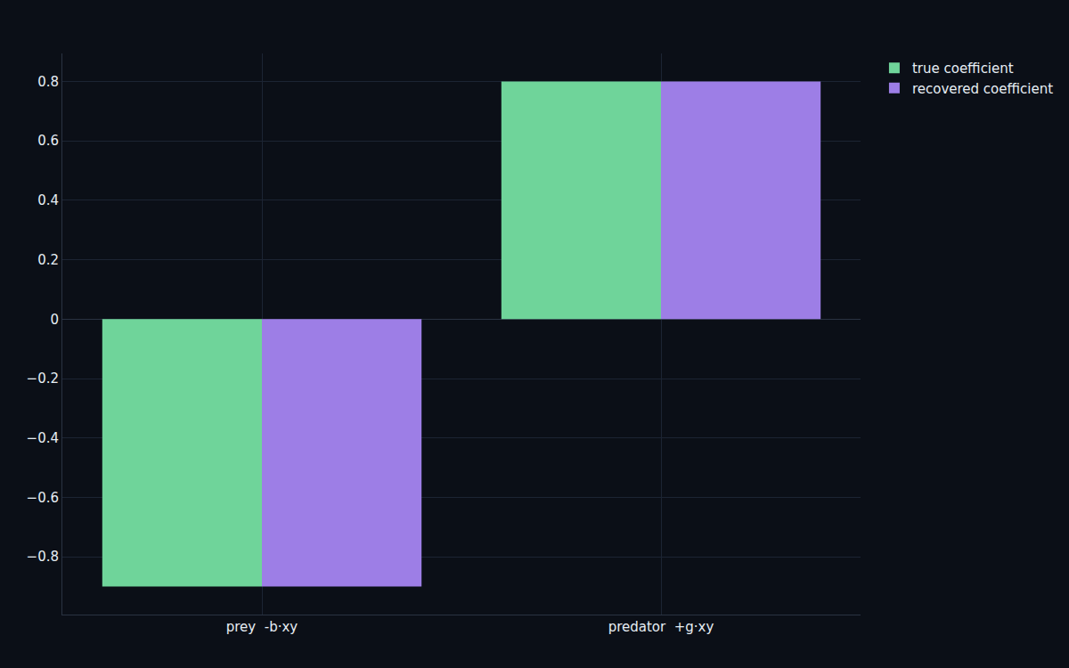
A discovered law generalizes; a fit does not.
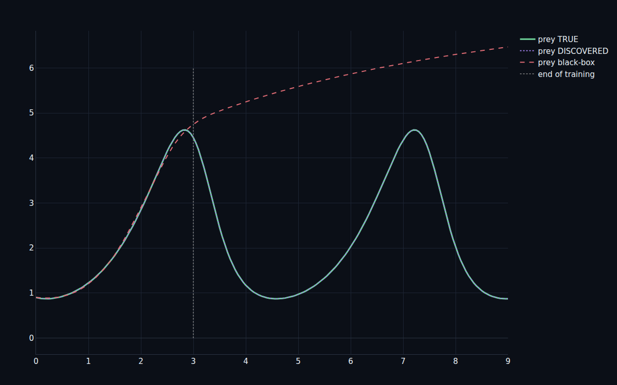
Because the UDE recovered the actual missing physics, the discovered symbolic model forecasts three times past the training window with zero error while the black-box neural ODE diverges — the difference between memorizing a window and learning a dynamics. The same pipeline recovers a damped Duffing oscillator's cubic stiffness term exactly, and the x·y recovery stays under 1% error through 10% measurement noise. Different systems, same workflow: keep what you know, learn the gap, read it back.
Every number re-derived from scratch at sign-off.
The V&V notebook retrains the UDE, re-runs the symbolic recovery, trains a fresh black-box baseline for the contrast, and re-runs the noisy recovery — then prints a PASS/FAIL board.
| Result | Requirement | |
|---|---|---|
| UDE hybrid-model fit RMSE | 0.065 | R-01 < 0.10 |
| Learned-term correlation | 0.926 | R-02 > 0.9 |
| Symbolic recovery error | 0.0% | R-03 < 10% |
| Extrapolation vs black box | ratio 0.0 | R-04 < 1/3 |
| Noisy recovery (2% noise) | 0.2% | R-05 < 25% |
A method showcase on textbook systems.
The deliverable is ten notebooks and the dossier — no custom blocks or canvases, because UDE discovery is a data-driven workflow, not an acausal network. The systems are deliberately small and didactic (2-state Lotka-Volterra, a Duffing oscillator) so the discovery payoff is legible; real closures — turbulent fluxes, reaction networks, constitutive laws — are higher-dimensional and need larger libraries and more data. The headline recovery is exact on clean data; the noise notebook shows graceful, not magical, degradation. The polynomial library is a fixed, small basis chosen a priori, and training is single-shooting. All of this is in the dossier's Honest Scope — and the whole thing runs on the Julia SciML stack (OrdinaryDiffEq · SciMLSensitivity · Lux · Zygote), a concrete reason to reach for it over MATLAB here.
Discover the missing physics in your own model.
Book a walkthrough and we'll set up your known model, the unknown channel, and run the UDE training and symbolic recovery on your data live.