
A motor switches at 20 kHz. Control has to make that smooth.
Power electronics is brutal at the bottom and elegant at the top. At the bottom, a converter chops DC on and off thousands of times a second and a motor is a tangle of cross-coupled three-phase currents. At the top, field-oriented control turns that into two clean knobs — torque and flux — you can command independently. This program walks the whole stack: the switching converter, the averaged model you design on, the dq machine, the FOC that decouples it, the PWM that realizes it, and the cascade speed loop that drives a load.
Everything starts as a square wave.
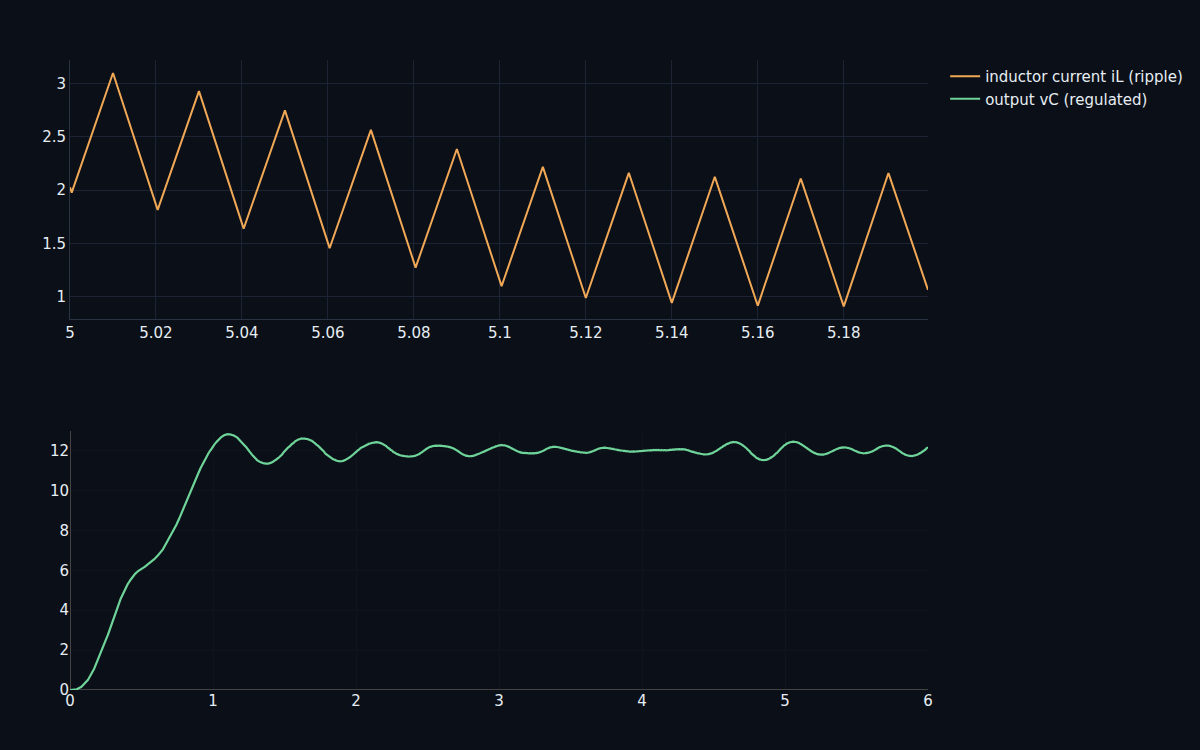
A buck converter regulates voltage by switching — full-on, full-off, thousands of times a second — and letting an inductor and capacitor average the result. The switched simulation shows the real thing: a triangular inductor-current ripple riding on the DC, and an output that settles to its setpoint within 0.034%. This is the raw material; every smooth quantity higher up is a controlled average of something that's actually chopping.
A three-phase motor's currents fight each other.
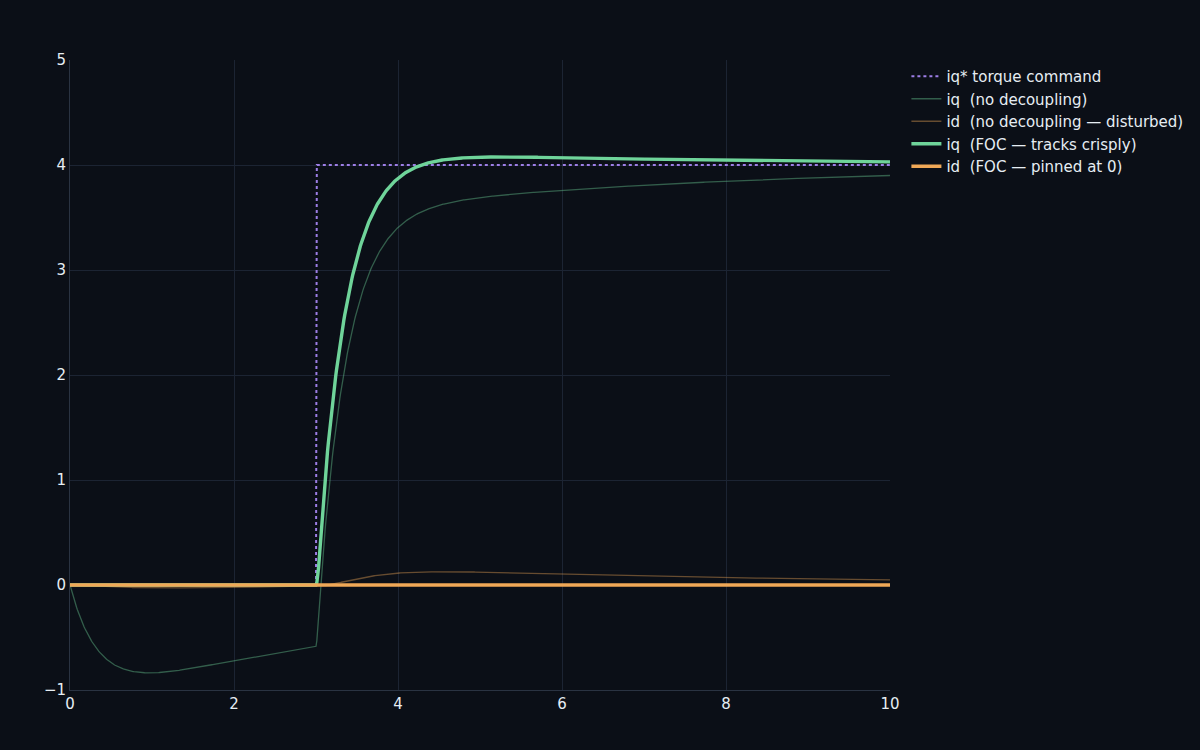
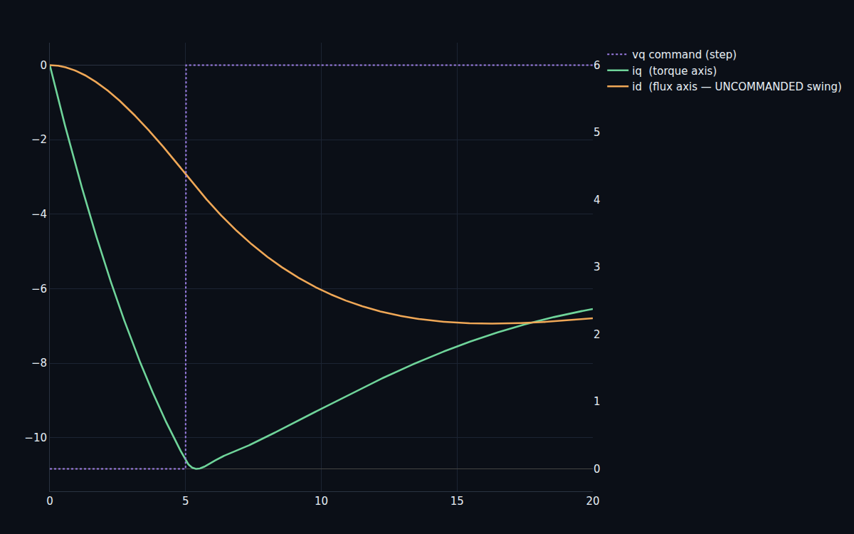
Transform the machine into the rotating dq frame and a spinning three-phase motor becomes two currents: id (flux) and iq (torque). But they're cross-coupled — command a torque-producing voltage and the flux current gets stirred along with it, and vice versa. Open-loop, a step in one axis disturbs the other by several amps. You can't independently set torque without first untangling that coupling.
Turn the voltage command back into switching.
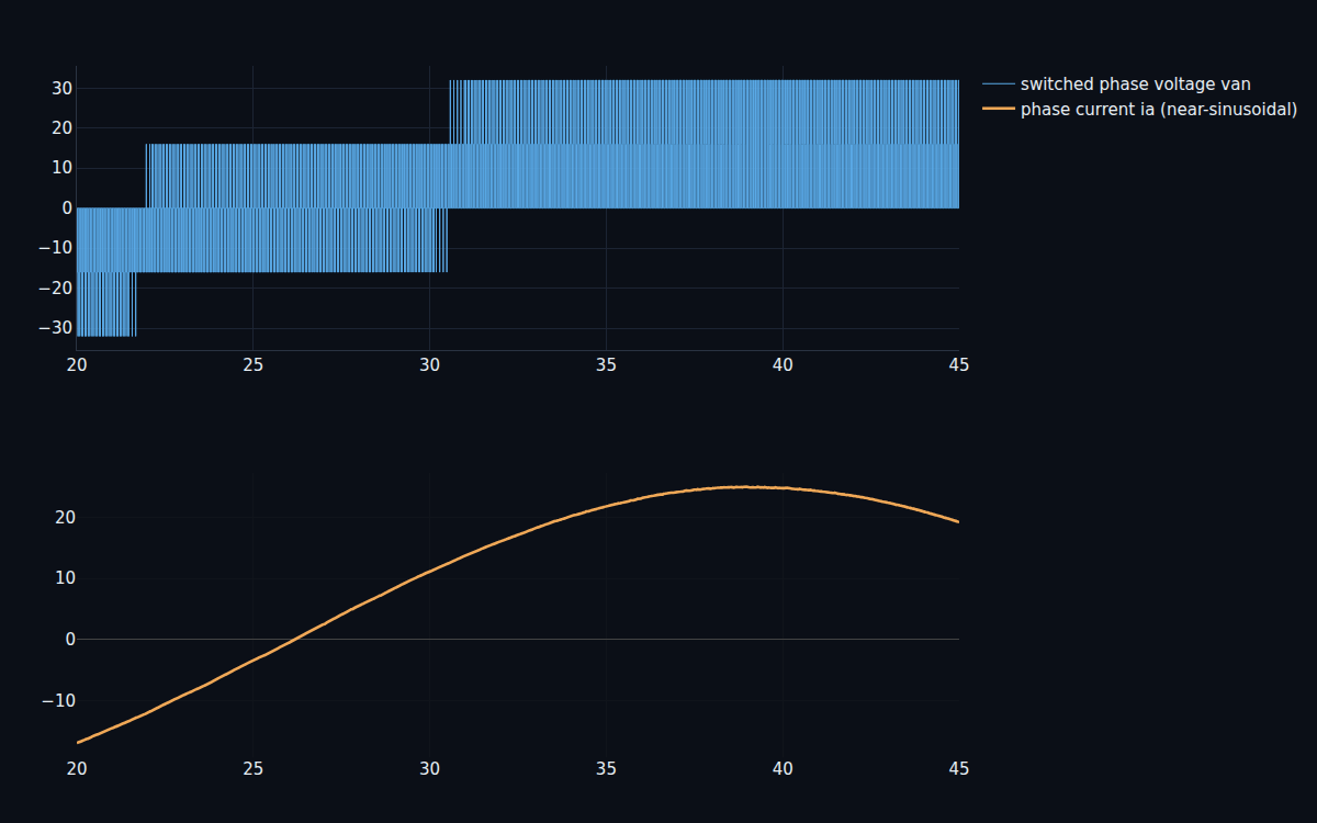
The controller computes a smooth dq voltage; the inverter can only switch. Inverse-Park plus carrier PWM turns the command into the actual on/off pole voltages, and the motor's inductance averages them back into a near-sinusoidal phase current. The smooth current the controller assumed and the chopped voltage the hardware delivers are two views of the same thing — the PWM is the bridge between them.
Wrap a speed loop around the torque.
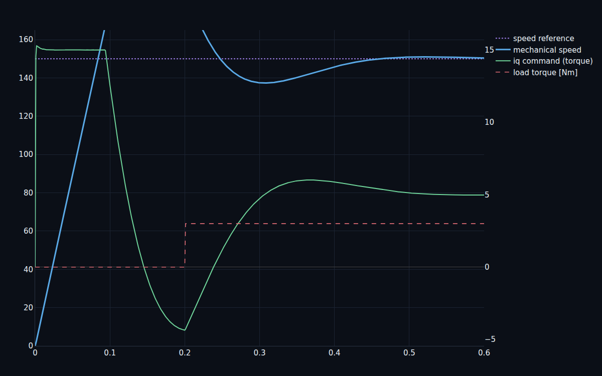
Torque control is the inner loop; a real drive commands speed. A cascade adds an outer speed PI that asks the FOC torque loop for exactly the torque needed — so the motor tracks a speed reference and shrugs off a load-torque disturbance (a 3 N·m step recovers to 0.285% residual). Past base speed, field weakening drives the flux current negative to trade torque for range, extending usable speed well past where a fixed-flux drive runs out — at a rated efficiency of 96%.
Every number re-derived at sign-off.
The V&V notebook rebuilds the converter, machine and controllers from scratch and re-derives the requirements, printing a PASS/FAIL board.
| Result | Requirement | |
|---|---|---|
| Buck output regulation | 0.034% | R-01 < 2% |
| Averaged-model fidelity | 0.257 V RMS | R-02 < 0.5 V |
| FOC torque-step decoupling | iq 0.74% / id 0 A | R-03 |
| Speed-loop load rejection | 0.285% | R-04 < 2% |
| Rated efficiency | 96.0% | R-05 > 88% |
Ideal switches, real control.
The deliverable is ten notebooks and the dossier — the models are switched ODEs with callbacks, not an acausal network. The switches are idealized (no device-level conduction/switching-loss physics beyond a lumped model), the thermal model is lumped, sensors are ideal with no estimation delay, and the PWM is carrier/sinusoidal rather than full space-vector with dead-time; the exact FOC decoupling is helped by the machine being non-salient. What the program does deliver is the complete drive stack — converter, averaging, dq machine, FOC, PWM, cascade speed control, field weakening — on reproducible numbers, the inverter-and-control layer one level below the EV-vehicle flagship.
Design your own motor drive.
Book a walkthrough and we'll set up your converter, machine and control loops, and run the switching, FOC and drive-cycle studies live.