
Watch a wave obey Maxwell's equations, cell by cell.
Electromagnetic fields fill space and evolve by Maxwell's equations — and you can solve them directly on a grid, letting the electric and magnetic fields leapfrog through time in step. That's the Finite-Difference Time-Domain method, the workhorse of computational electromagnetics (HFSS, CST, COMSOL-RF). This program builds an FDTD solver from scratch and uses it to reproduce, one notebook at a time, the wave phenomena every physics course teaches: a wave radiating, refracting, diffracting, scattering, and resonating. It's the field-solver sibling to the CFD flagship.
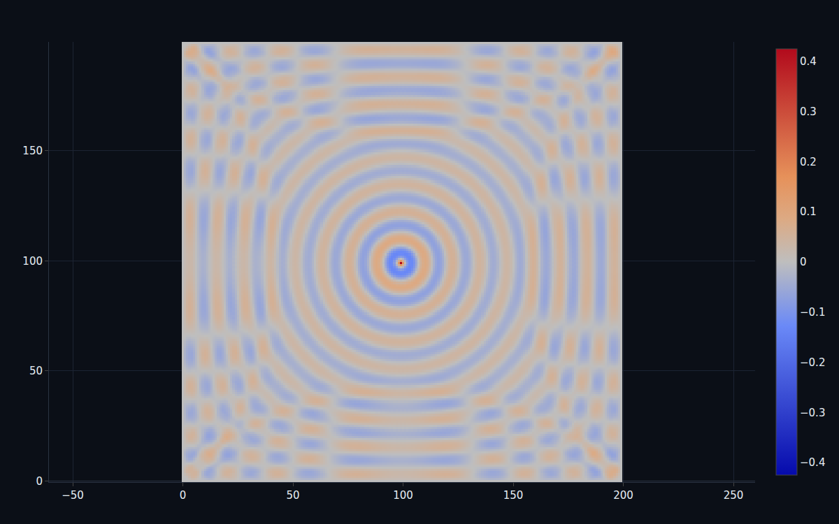
Two curl equations, leapfrogging on a staggered grid.
Maxwell's curl equations say a changing magnetic field makes an electric one and vice versa. FDTD discretizes them on the Yee grid — electric and magnetic field components interleaved in space and updated alternately in time — so the simulation literally marches the wave forward. The one rule you can't break is the Courant stability limit: step too far per tick and the field explodes. Get it right and a point source radiates clean circular wavefronts at exactly the speed of light.
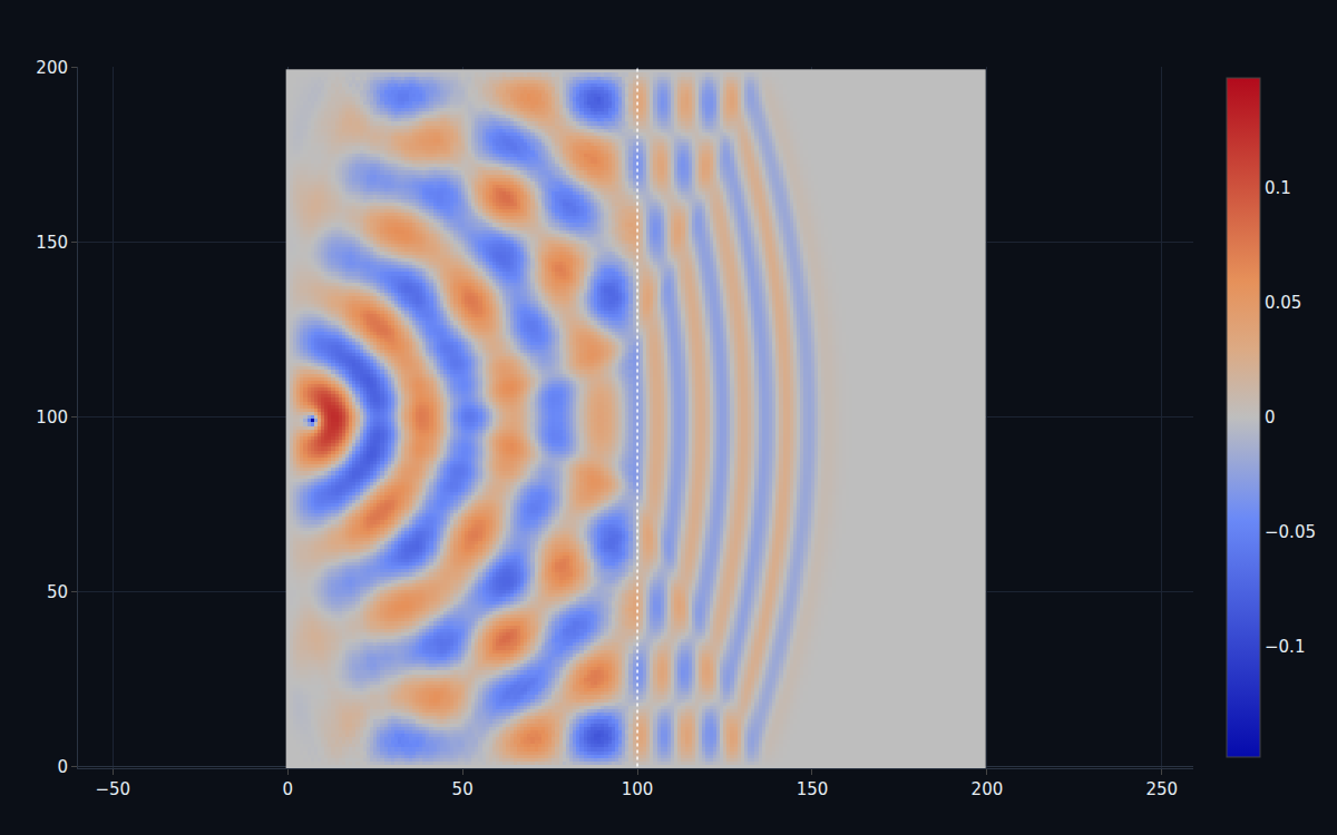
Put glass in the path and the wave slows and bends.
Drop a region of higher permittivity — glass, water, any dielectric — into the grid and the wave slows down inside it. Part of it reflects at the interface, part transmits with a compressed wavelength, and the ratio of wavelengths is exactly the refractive index √εr — Snell's law, emerging from the field update with no law of refraction coded in. The solver reproduces it to a couple percent, dispersion error and all.
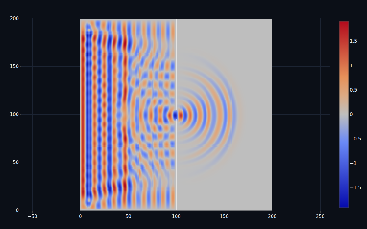
A conductor casts a shadow and scatters the rest.
Send a plane wave at a conducting cylinder and two things happen at once: a standing-wave pattern builds up in front as the incident and reflected waves interfere, and a quiet shadow forms behind. Scattering and shadowing are how radar sees, how an antenna's surroundings distort it, and how a stealth shape is judged — and they come straight out of forcing the field to zero on the conductor.
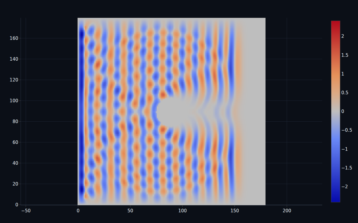
Close the box and only certain notes survive.
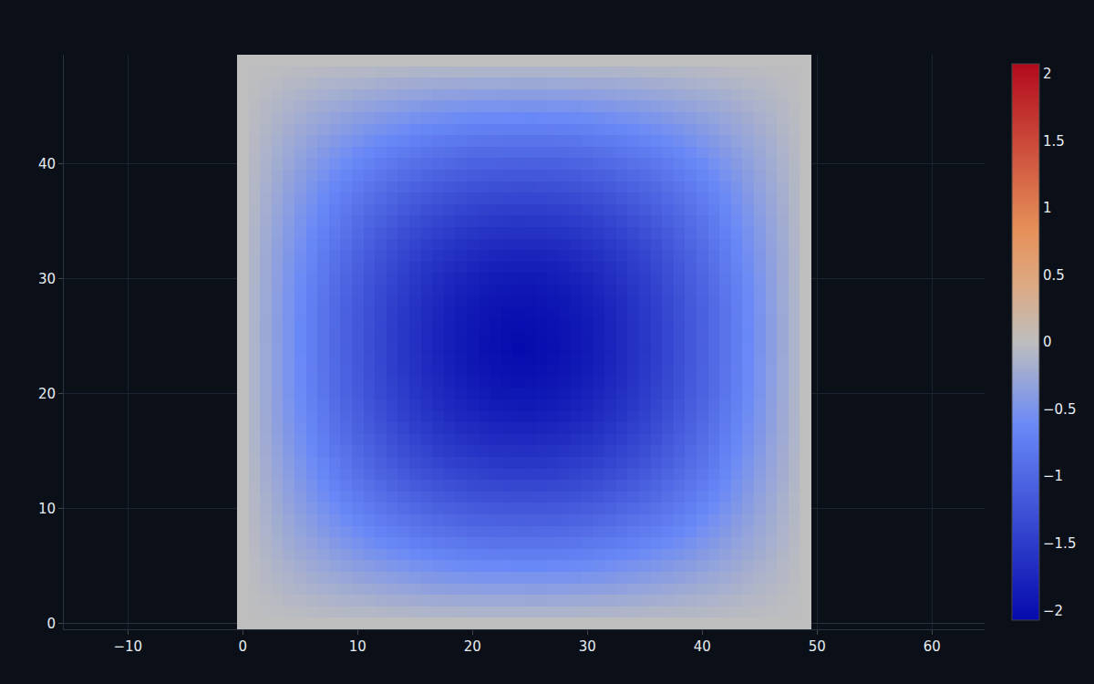
Trap the field in a conducting box and it can't radiate away — instead it rings at the cavity's resonant frequencies, the electromagnetic equivalent of an organ pipe's notes. Drive a broadband pulse and Fourier-transform the response, and the spectrum peaks land on the analytic cavity modes to within half a percent; drive it at a resonance and the corresponding standing-wave mode pattern fills the box. Resonators, filters and waveguides all live on this physics.
Every number re-derived at sign-off.
The V&V notebook rebuilds the solver from scratch and re-derives each requirement against theory, printing a PASS/FAIL board.
| Result | Requirement | |
|---|---|---|
| Wave speed (magic step) | 1.000 | R-01 = 1.000 |
| Courant stability | bounded | R-02 |
| Wavelength vs c/f | +3.7% | R-03 |
| Snell index vs √εr | 2.05 vs 2.00 | R-04 |
| Cavity resonance | 0.5% | R-05 |
A real field solver, at teaching fidelity.
The deliverable is ten notebooks and the dossier — a discretized Maxwell field, not an acausal lumped network, so there's no custom block or canvas. The solver is 2D (transverse-magnetic), in normalized units, at modest grid resolution — so there's measurable numerical dispersion, the cylinder and screens use staircase conducting boundaries, the absorbing boundary is a tapered lossy rim rather than a full split-field PML, and the media are non-dispersive and linear. What the program proves is the capability the portfolio lacked alongside CFD — solving Maxwell's equations as a field on a grid — with a self-contained solver (no external EM dependency) that reproduces radiation, refraction, diffraction, scattering and resonance, every number re-runnable and checked against theory. It pairs naturally with the SAR radar flagship.
Simulate your own electromagnetic problem.
Book a walkthrough and we'll set up your geometry, materials and sources, and run the field solve, scattering and resonance studies live.