
Cart-pole, from textbook to reinforcement learning.
A pole hinged on a cart, the cart pushed by a horizontal force — the benchmark every controls course starts with, and the one every RL paper returns to. Here it is one program: the exact nonlinear dynamics, a full-state LQR that catches the inverted pole, an energy-shaping swing-up, a learned model-free policy, and a Monte-Carlo robustness sign-off — the plant and its stabiliser also composed as one runnable .djl on the canvas.
Five ways to balance one pole.
From a hand-derived model to a policy that learns with no model at all — each method is its own runnable notebook, all on the same plant.
Nonlinear dynamics
The exact cart-pole equations of motion, derived and integrated. The upright equilibrium is genuinely unstable — ∂θ̈/∂θ > 0 — so every uncontrolled run topples, the right baseline to beat.
LQR stabilisation
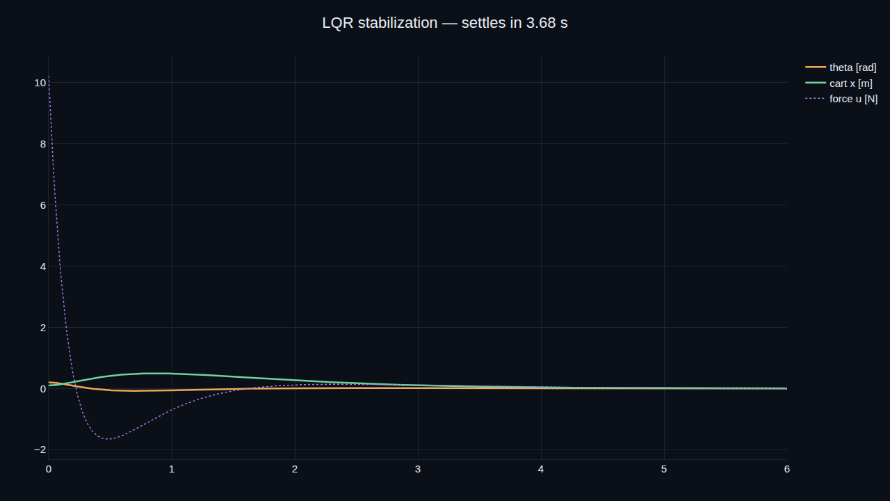
A full-state feedback law from lqr(A, B, Q, R) pulls every closed-loop eigenvalue into the left half-plane and settles an 11° lean to upright in 3.68 s.
Energy swing-up
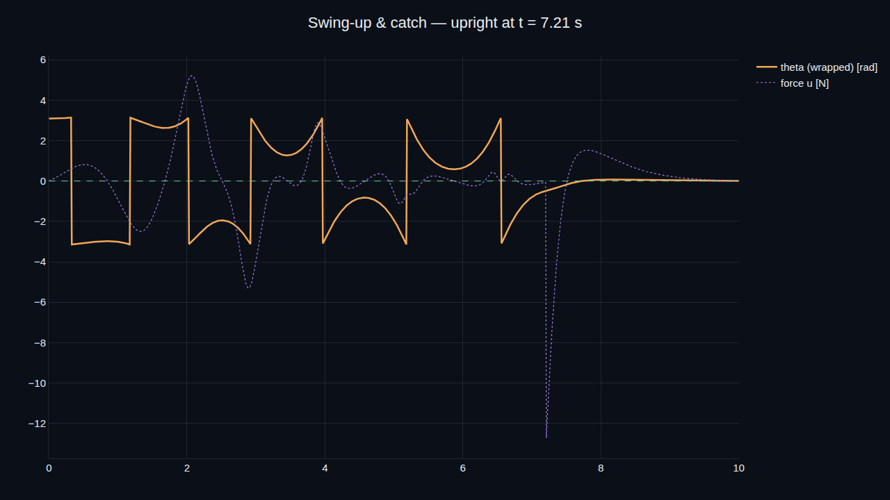
An energy-shaping law pumps the pole from hanging all the way around, then hands off to LQR, which catches it upright at t ≈ 7.2 s.
Reinforcement learning
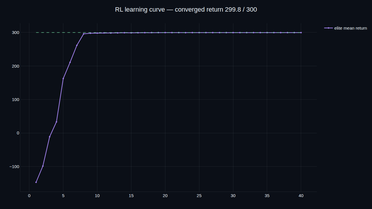
A cross-entropy-method policy learns to balance from random initial conditions with no model — converging to 299.6/300 return from a −220 random baseline.
Robustness
A 300-trial Monte-Carlo sweep perturbs cart mass, pole mass and length by ±30% and kicks the pole with impulses — all 300 are caught.
Gain optimisation
A bounded Nelder-Mead search retunes the LQR weights against a closed-loop cost, cutting it 34.5% while the gains stay physical.
The plant and its controller, composed on a canvas.
The whole closed loop — the nonlinear cart-pole plant and its full-state LQR law — is one acausal .djl component. Its equations are written implicitly in the accelerations ẍ and θ̈, a small algebraic system the kernel solves every step, so it is a genuine differential-algebraic model that needs a stiff Rodas5P solver, not a hand-rolled time-step. It lowers and runs through the same production engine the canvas uses: released from a 0.20 rad lean, the controller drives the pole to 0.005 rad. The gains are the same lqr() values the notebooks compute.
Every result is a number you can re-run.
Each notebook is gated on its own worker-verified result, and the .djl stabiliser is confirmed solving through the production canvas engine.
| Result | Detail | |
|---|---|---|
| LQR settling time | 3.68 s | all poles in LHP |
| Swing-up catch | t ≈ 7.2 s | θ → 0.0018 rad |
| Learned RL return | 299.6 / 300 | −220 baseline |
| Q/R optimisation | −34.5% cost | bounded search |
| Robustness caught | 300 / 300 | ±30% params |
A benchmark, done honestly.
The pole is a point-mass pendulum on a frictionless cart — the standard textbook cart-pole, not a flexible or multi-body arm. The reinforcement-learning policy is a linear cross-entropy method chosen for speed and reproducibility, not a deep network; the optimiser is a bounded local search. What the program shows is the full arc — derive, stabilise, swing up, learn, and verify — on one plant, with the controller also living as composable acausal source you can wire into a larger system.
Bring your own plant.
Book a walkthrough and we'll stand up your dynamics, design the controller, and run the swing-up, learning and robustness studies live.