
The honest answer is a distribution, not a number.
Every other model in this portfolio gives one answer. But fit a model to noisy data and the right answer isn't "the rate is 0.7" — it's "0.7, and here's exactly how sure I am." Bayesian inference produces that: a full posterior distribution over the parameters, and calibrated uncertainty on every prediction. Markov-Chain Monte Carlo is the engine. This program builds it from the conjugate case you can check by hand up through calibrating a dynamical model and comparing competing ones — and it complements every other flagship, because uncertainty can wrap any of them.
Start where you can check the answer exactly.
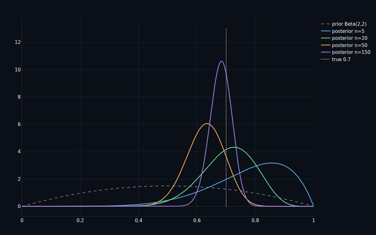
For some models the posterior is analytic — a Beta prior and binomial data give a Beta posterior, in closed form. The program starts there, watching the posterior sharpen onto the true value as data arrives, because it's the case where a sampler can be validated to the last digit. Get the machinery right where you can verify it, then trust it where you can't.
A fit you can't doubt is a fit you can't trust.
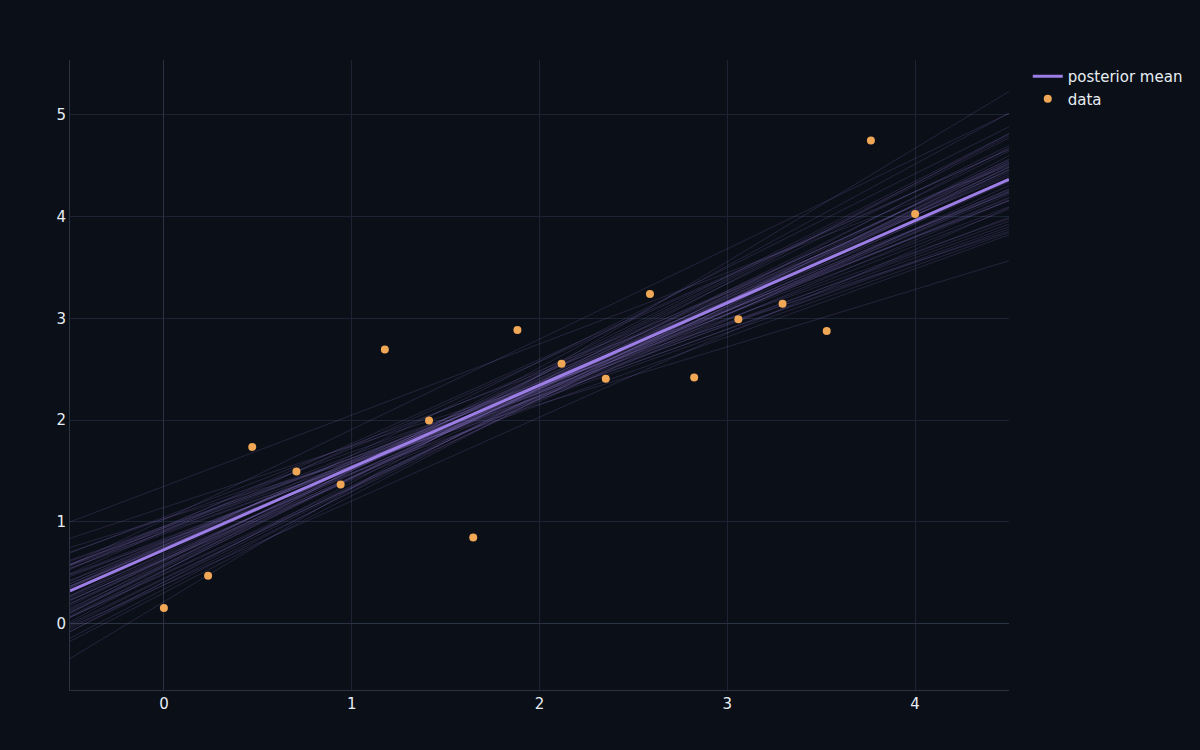
Least-squares draws one line through the data and stops. Bayesian regression draws the whole posterior over lines — and the spread of that fan, narrow where data is dense and flaring where it's sparse, *is* the uncertainty. That's the difference between a prediction and a prediction you can act on: not just the best guess, but how far it might be off, everywhere.
Calibrate a dynamical model — with error bars.
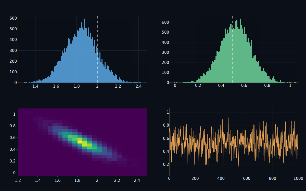
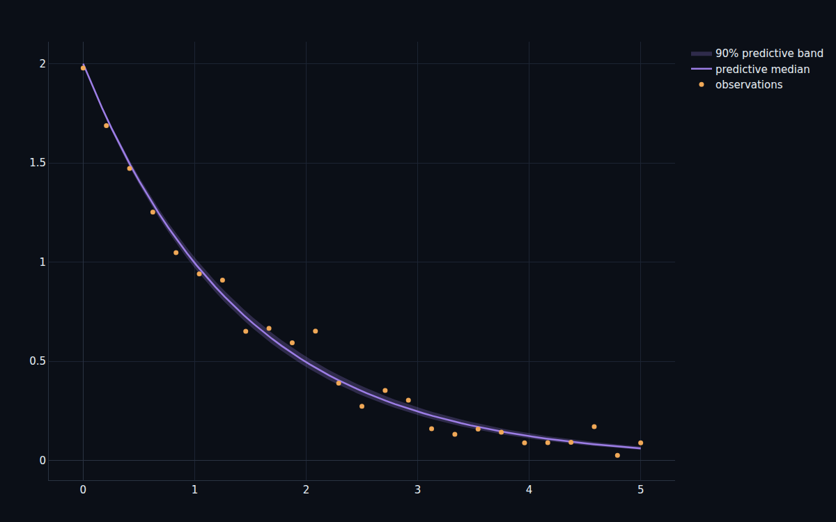
The same machinery infers the parameters of an ODE. Given noisy observations of a decaying signal, MCMC recovers the decay rate as a posterior (centred on the truth), and pushing that posterior forward through the model produces a posterior-predictive band — a forecast that carries its own uncertainty. And the program checks that the uncertainty is honest: across many replications, the 90% credible intervals contain the truth about 90% of the time. Calibration, verified.
Let the data pick the model — and punish complexity.
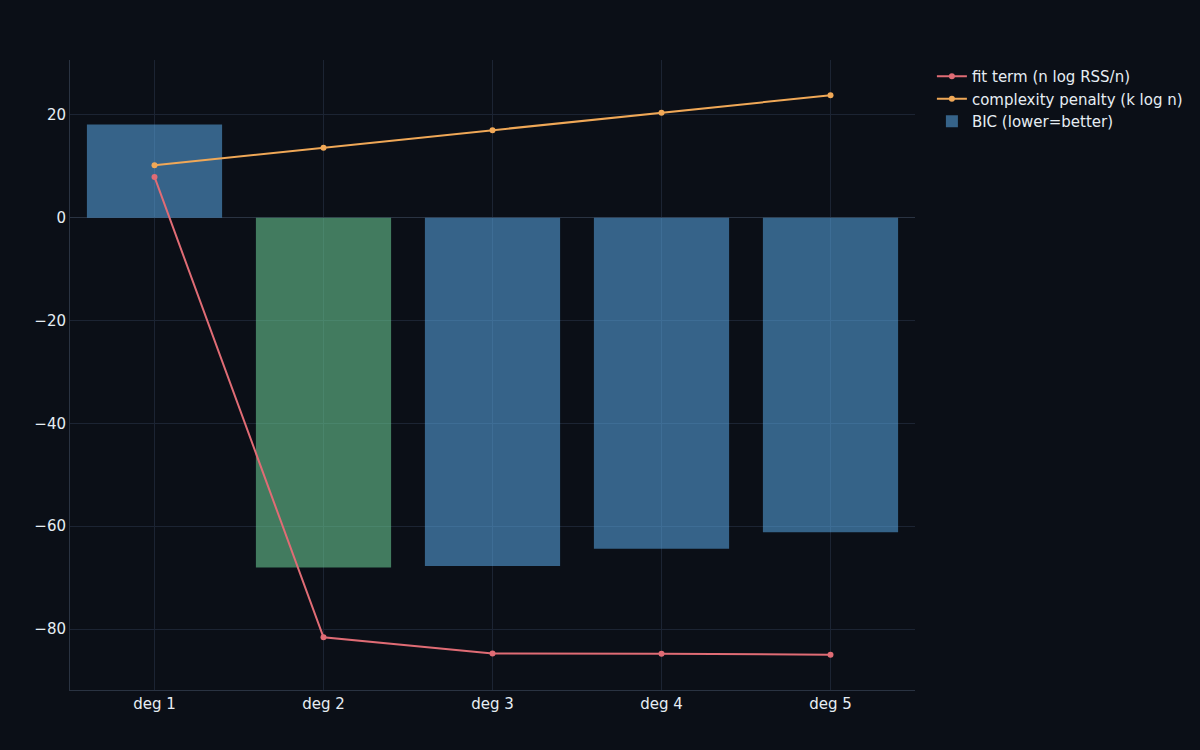
Given competing models — a straight line versus a parabola — which does the data support? A more complex model always fits the training data better, so the honest comparison penalizes complexity. The Bayesian information criterion does exactly that, and over a sweep of polynomial degrees it bottoms out at the true degree: enough flexibility to fit the signal, no more. Occam's razor, made quantitative.
Every number re-derived at sign-off.
The V&V notebook rebuilds each sampler from scratch with fixed seeds and re-derives the requirements against theory, printing a PASS/FAIL board.
| Result | Requirement | |
|---|---|---|
| MCMC vs analytic posterior | mean diff 0.002 | R-01 |
| Parameter recovery (CI ∋ truth) | 1.85 / 0.53 | R-02 |
| Multi-chain R̂ | 1.001 | R-03 ≈ 1 |
| Predictive-interval coverage | 86% | R-04 ≈ 90% |
| Model comparison (BIC) | true degree | R-05 |
The sampling paradigm, anchored to theory.
The deliverable is ten notebooks and the dossier — MCMC samplers and posteriors, not an acausal network, so there's no custom block or canvas. The sampler is random-walk Metropolis–Hastings (not gradient-based HMC/NUTS), likelihoods are Gaussian, chains are modest length, the models are low-dimensional, model comparison uses an information criterion rather than a full marginal likelihood, and nothing is calibrated to a real-world dataset. What the program proves is the Bayesian paradigm itself — a distribution over answers with calibrated uncertainty — validated against closed-form posteriors where they exist, and reaching dynamical-model calibration, uncertainty propagation, and model comparison where they don't. It is the uncertainty layer that can wrap any other flagship.
Quantify the uncertainty in your own model.
Book a walkthrough and we'll set up your model and data, run the MCMC, and produce calibrated posteriors and predictive bands live.