
Plan the mission. Optimise the fleet. Fly it — in simulation.
A LiDAR survey of a 500 × 500 m site near Al-Batinah South, Oman, taken from a brief to an optimal, flyable mission entirely in DjiniousLab. Drone, LiDAR and fleet specs drive a coverage plan; an optimiser tunes altitude, speed and fleet allocation to whatever you care about — fastest, fewest battery swaps, or highest resolution; a Python mission then commands a simulated UAV fleet, replayed on an animated map. Six notebooks, one workflow, all on the worker.
From a site brief to a flyable mission, in six steps.
Each step is a Python notebook running on the DjiniousLab worker — numpy/scipy for the planning maths, Plotly and Leaflet for the maps. Nothing is hard-coded: change a spec and the whole mission re-plans.
Site & datum
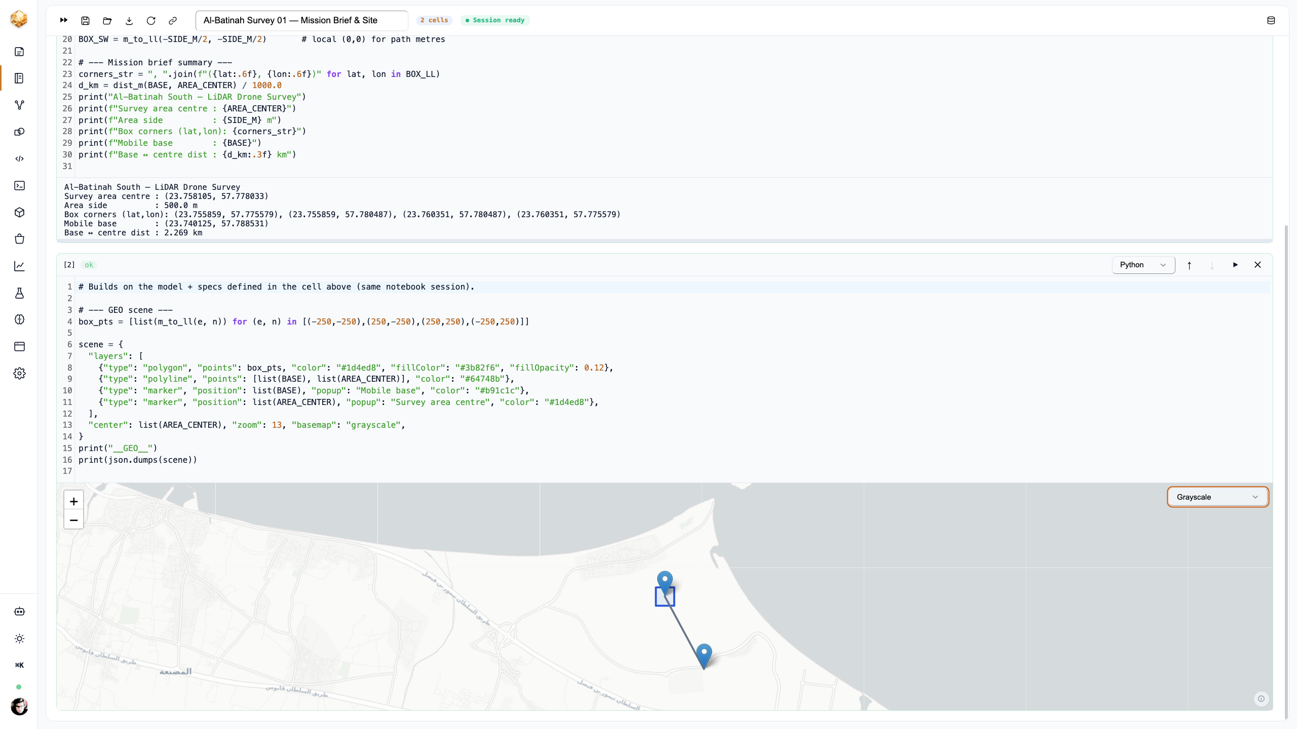
The 500 m survey box and a mobile launch base are pinned in WGS-84 over the real Al-Batinah coastline. A local east-north metre frame (equirectangular at the site latitude) carries all the geometry; base-to-area transit comes out at ~2.3 km — and it is charged against every sortie's endurance.
Drone & LiDAR spec model
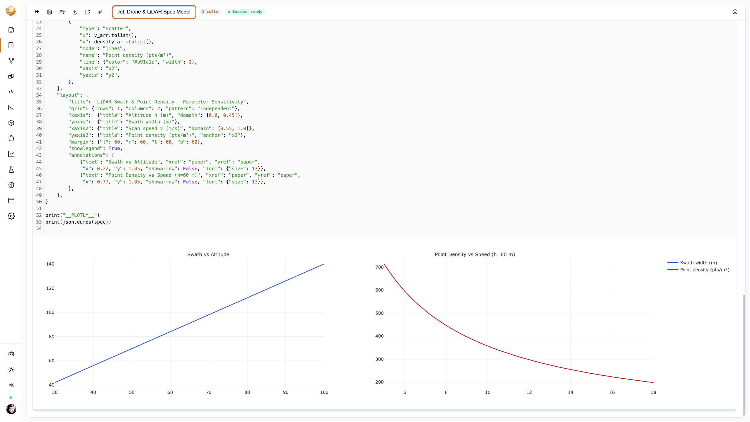
Cruise/scan speed, battery endurance and turnaround for the drone; field-of-view, point rate and minimum altitude for the LiDAR. Ground swath = 2·h·tan(FOV/2) and point density = rate / (swath · speed) fall straight out — so altitude and speed trade coverage against resolution.
Coverage path
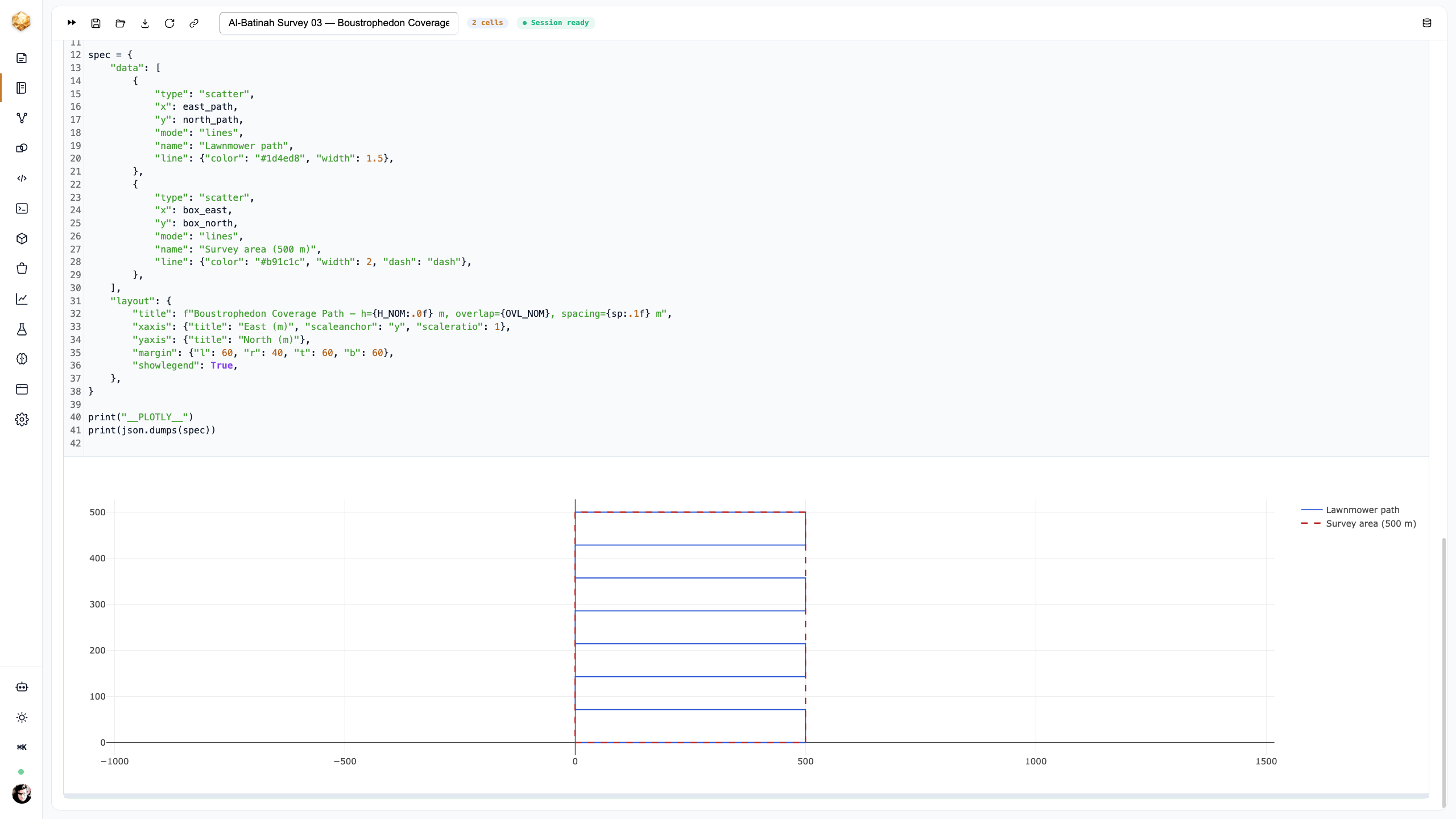
A boustrophedon (lawnmower) path tiles the box at the swath spacing implied by the chosen altitude and overlap. At 60 m and 20 % overlap that is an 84 m swath, ~8 lines and a 4.5 km scan path — the raw work the fleet has to share.
Fleet allocation & optimisation
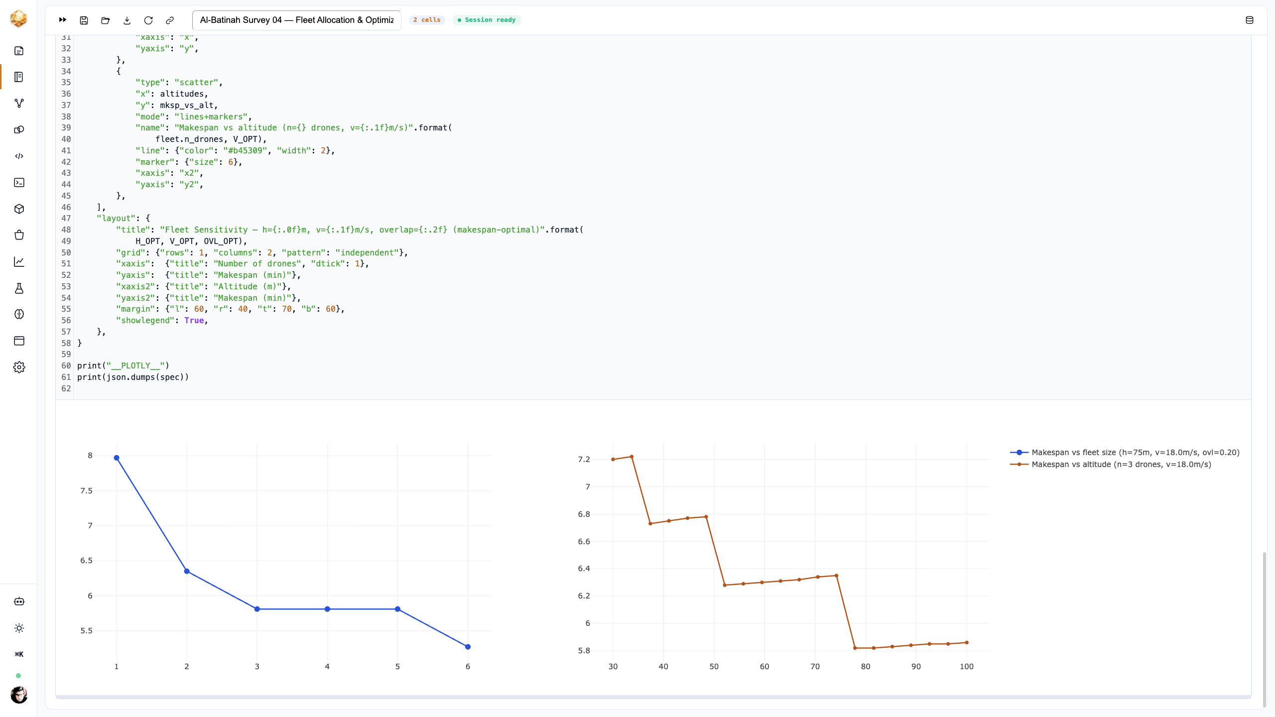
The strips are split into contiguous bands flown concurrently, so adding drones genuinely cuts the makespan. A sweep over altitude, speed, overlap and fleet size finds the optimum for the chosen objective — and shows the trade: makespan drops 34 % going from one drone to six.
Python mission → simulated fleet
The optimal plan becomes a per-drone waypoint program. A pure-Python driver commands a simulated remote fleet — arm, take off, go-to, scan, return — streaming live telemetry and a progress bar. The radio link is faked; the command structure reads exactly like the real thing.
Animated mission map
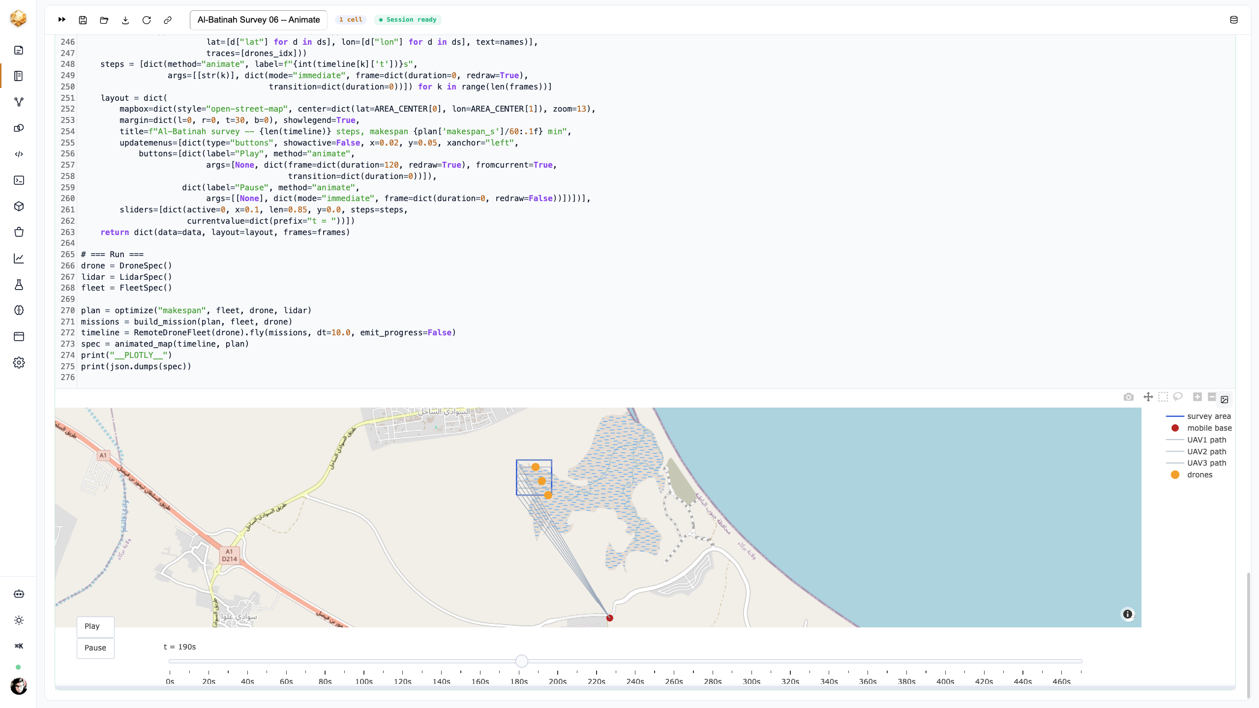
The telemetry timeline replays on an OpenStreetMap basemap: three UAVs launch from the base, transit, scan their bands concurrently and return, with a play button and time-scrubber over 48 frames. The headline artefact a planner can actually watch.
Specs in, mission out — change one number and re-plan.
The mission is a function of the hardware, not a fixed plan. The drone's endurance sets how much of the survey fits in one sortie; the LiDAR's field-of-view and point rate set how wide each pass is and how dense the returns are; altitude and speed trade the two off against each other. Because every downstream step reads these specs, swapping in a different drone or sensor — or relaxing the overlap — re-derives the swath, the path, the sortie count and the optimal fleet automatically. The plots below are the levers a planner actually turns.
- Ground swath grows linearly with altitude; point density falls with altitude and speed.
- Endurance minus the ~2.3 km round-trip transit sets the per-sortie scan budget.
- Overlap, altitude and speed are the continuous knobs the optimiser sweeps.
One model. Three objectives. You choose what 'optimal' means.
The same plan can be optimised three ways: minimise mission time (makespan), minimise battery sorties, or maximise LiDAR resolution within a time budget. The fleet flies concurrently — strips split into contiguous bands — so the makespan objective genuinely rewards more drones, while the resolution objective drives the altitude down at the cost of time. A sensitivity sweep over fleet size and altitude makes the trade visible, so the choice is an engineering decision, not a guess.
- Concurrent banding: makespan = the busiest drone's wall-time, so a bigger fleet finishes sooner.
- Makespan falls from 8.0 min (1 drone) to 5.3 min (6 drones) at the time-optimal altitude.
- Resolution-first pushes altitude to its floor — higher point density, longer mission.
Three objectives, three missions.
The same 500 m survey, optimised three ways for the default UR-class fleet. Minimising time flies high and fast; maximising resolution flies low and slow. (Here, fewest-sorties and best-resolution coincide at the altitude floor.)
| Altitude | Mission time | LiDAR density | |
|---|---|---|---|
| Minimise mission time | 75 m | 5.8 min | ≈159 pts/m² |
| Fewest battery sorties | 30 m | 13.0 min | ≈1 322 pts/m² |
| Maximise resolution (≤ 90 min) | 30 m | 13.0 min | ≈1 322 pts/m² |
A planning digital twin, not a flight system.
Everything here is simulation. The UAV fleet is faked — there is no radio link or autopilot; the Python driver mimics a real go-to/telemetry command interface but talks to a stub. The flight model is planning-grade: flat ground, no wind, a simplified energy budget, and an optimum found within the swept parameter ranges. What it is good for is exactly what a mission planner needs before anyone flies: sizing the fleet, choosing the altitude and speed, and seeing the time/resolution trade-off — on a real site, with your own drone and sensor numbers, in minutes.
Plan your own survey.
Book a walkthrough and we'll drop in your site, drone and LiDAR specs and optimise the mission live.